Model evaluation

The cloudnetpy.model_evaluation subpackage connects Cloudnet observation products with the corresponding fields simulated by numerical weather prediction (NWP) models, and brings them onto a common grid so that they can be compared directly. The goal is to highlight the capabilities and shortcomings of simulated cloud variables against ground-based remote sensing observations.

Comparing observations with a model is not trivial: the two live on very different grids. Cloudnet products have a fine time-height resolution (typically ~30 s and ~30 m), while a model column is coarse in the vertical and represents a grid-box average in the horizontal that a point measurement only samples as air advects past the site. The subpackage handles this by downsampling the high-resolution observations onto the model grid, producing so-called L3 day-scale products: a single file holding 24 hours of the model’s own fields next to the regridded observation fields.

Day-scale products are the building block of the model evaluation. Climatological products for longer time scales (month, season, year, etc.) are intended to be aggregated from the day-scale products at a later stage.

Inputs

Each L3 product is generated from two files:

• A Cloudnet observation file — the categorize file for cloud fraction (the cloud mask is built from its category bits), or an iwc or lwc product file. It must be processed with CloudnetPy so that the expected variables and category bits are present.

• A harmonized model file for a specified forecast range (e.g. steps 0h – 7h combined from consecutive model runs). All models are expected to share the same variable names and units (temperature [K], pressure [Pa], qi/ql ice/liquid mixing ratios and cloud_fraction [1], uwind/vwind [m s^-1], height [m]). The only quantity that genuinely differs between models is the number of vertical levels, which is derived dynamically from the model height and a fixed altitude limit (22 km — levels above this are dropped because the radar cannot observe them).

The model’s own fields are written with a model_ prefix; the downsampled observation fields are written without a prefix. The model identity is stored in the global attributes.

Processing overview

The day-scale processing of cloud fraction, ice water content and liquid water content follows the same chain:

1. Read the observation product and derive the observed quantity (ObservationManager).

2. Read the harmonized model file and derive the comparable model quantity (ModelManager).

3. For cloud fraction only, apply the cirrus filter advance method, which reduces the model’s high-cloud fraction to account for the radar’s inability to detect small ice crystals (AdvanceProductMethods).

4. Downsample the observation onto the model time-height grid, on both the standard grid and a wind-advection grid (ProductGrid).

5. Write the L3 netCDF file with both model and downsampled-observation fields.

The entry point is cloudnetpy.model_evaluation.products.product_resampling.process_L3_day_product().

Observation products

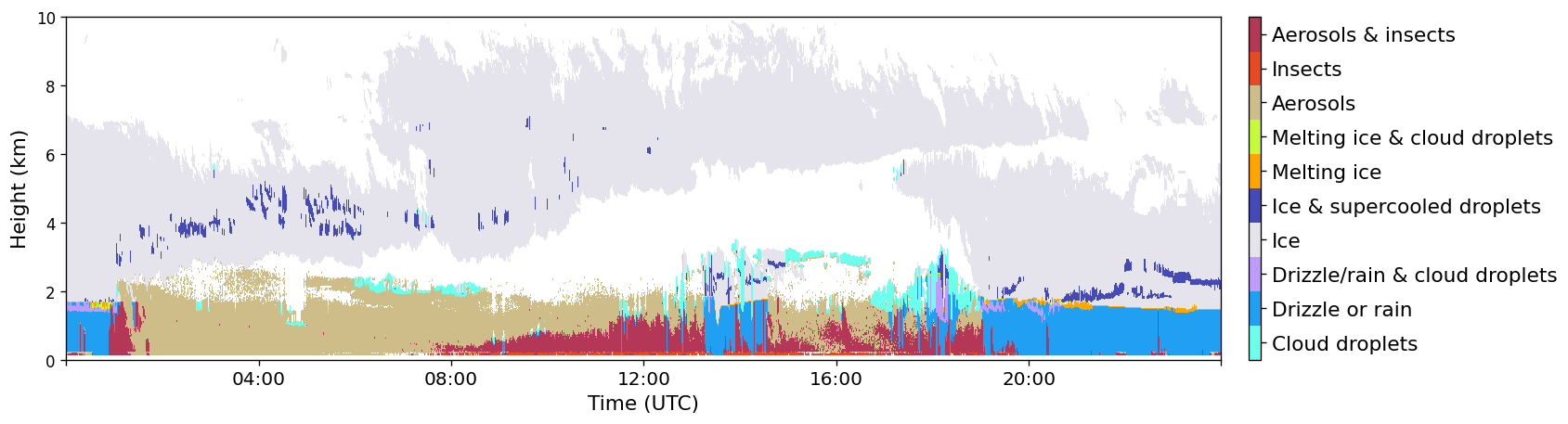
Cloudnet L2 product ‘Classification’. The underlying categorize bits are used to generate an ‘observed’ cloud fraction, since cloud fraction itself cannot be observed directly. Cloud fraction is a post-processed variable of models.

Cloud fraction (cf). Cloud fraction cannot be measured directly, so an observed cloud mask is built from the categorize category bits: droplet and (cold) falling-ice pixels are treated as cloud, while drizzle/rain, aerosol and insect pixels are treated as clear. The result is a binary cloud mask at the native observation resolution, which is later averaged into a fractional value when regridded.

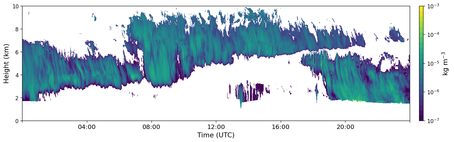
Cloudnet L2 product ‘Ice water content’. Models output the mixing ratio of ice; a comparable water content is derived from the model temperature, pressure and moisture.

Ice water content (iwc). The observed IWC is taken from the Cloudnet IWC product, keeping only reliable retrievals — retrieval status 1 (reliable) and 3 (radar corrected for liquid, rain and melting attenuation). Lidar-only, uncorrected-attenuation and rain-contaminated pixels are masked out.

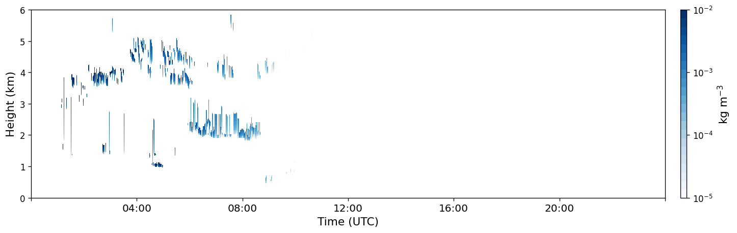
Cloudnet L2 product ‘Liquid water content’. As with IWC, a comparable model water content is derived from model fields.

Liquid water content (lwc). The observed LWC is read directly from the Cloudnet LWC product (scaled-adiabatic retrieval).

Model products

The model fields are made comparable to the observations:

• Cloud fraction is read directly from the model’s cloud_fraction variable; values below 0.05 are masked.

• Ice and liquid water content are not stored as such by models, which instead output a mixing ratio q at each grid point. The water content is computed from the ideal gas law, WC = q * p / (Rs * T), using the model pressure p and temperature T. For ice, the total frozen-condensate mixing ratio is used — the cloud-ice field qi plus any snow (qs) and graupel (qg) categories present — so that the model IWC includes precipitating ice and stays consistent with the observed IWC.

Downsampling to the model grid

The observation grid is always finer than the model grid, so observations are averaged into each model time-height cell (ProductGrid). The vertical cell edges are taken halfway between model levels; the time edges come from the model time steps.

Standard vs. advection grid. Each product is downsampled twice. The standard grid simply collects the observation pixels that fall within the model cell’s own time-height extent. The advection grid accounts for the fact that a model grid box represents a horizontal area, not a point: using the model wind speed and horizontal resolution, the time it takes for air to advect across one grid box is estimated, and the observation time window is widened (or narrowed) accordingly. Advection time is larger at upper levels where winds are stronger — a small effect in the mid-latitudes but visible in the tropics. Advection-grid variables carry an _adv suffix.

Cloud fraction: by volume vs. by area. For cloud fraction two averaging methods are produced from the binary cloud mask within each model cell:

• By volume (cf_V) — the mean over all observation pixels in the cell, i.e. the fraction of the cell volume that is cloudy.

• By area (cf_A) — the fraction of observation columns (profiles) that contain cloud at any height, i.e. a column counts as cloudy regardless of cloud depth.

IWC and LWC are downsampled by simple averaging of the valid (unmasked) pixels.

Cirrus filtering (cloud fraction advance method)

Radars struggle to detect the small ice crystals found in high cirrus, so a model can legitimately show cloud where the radar reports none. To make the comparison fair, the model cloud fraction is post-processed into an additional model_cf_cirrus field (AdvanceProductMethods). In ice-dominated cells the in-cloud IWC is converted to a gamma distribution of expected IWC (its variance estimated from the model wind shear and horizontal resolution), and the fraction of that distribution lying below the radar’s reflectivity sensitivity — derived from Z_sensitivity and the radar frequency via the Z–T relation — is removed from the model cloud fraction. The result is the model cloud fraction the radar would plausibly have been able to see.

Output L3 products

The L3 file holds the model’s own fields and the downsampled observations on the model’s grid. For cloud fraction:

Variable	Description
model_cf	Model cloud fraction
model_cf_cirrus	Model cloud fraction with cirrus filtering applied
cf_V / cf_A	Observed cloud fraction by volume / by area
cf_V_adv / cf_A_adv	Same, on the wind-advection time grid

For IWC and LWC:

Variable	Description
model_iwc / model_lwc	Model ice / liquid water content
iwc / lwc	Observed water content regridded by averaging
iwc_adv / lwc_adv	Same, on the wind-advection time grid

Example L3 day products — model simulation versus downsampled observation:

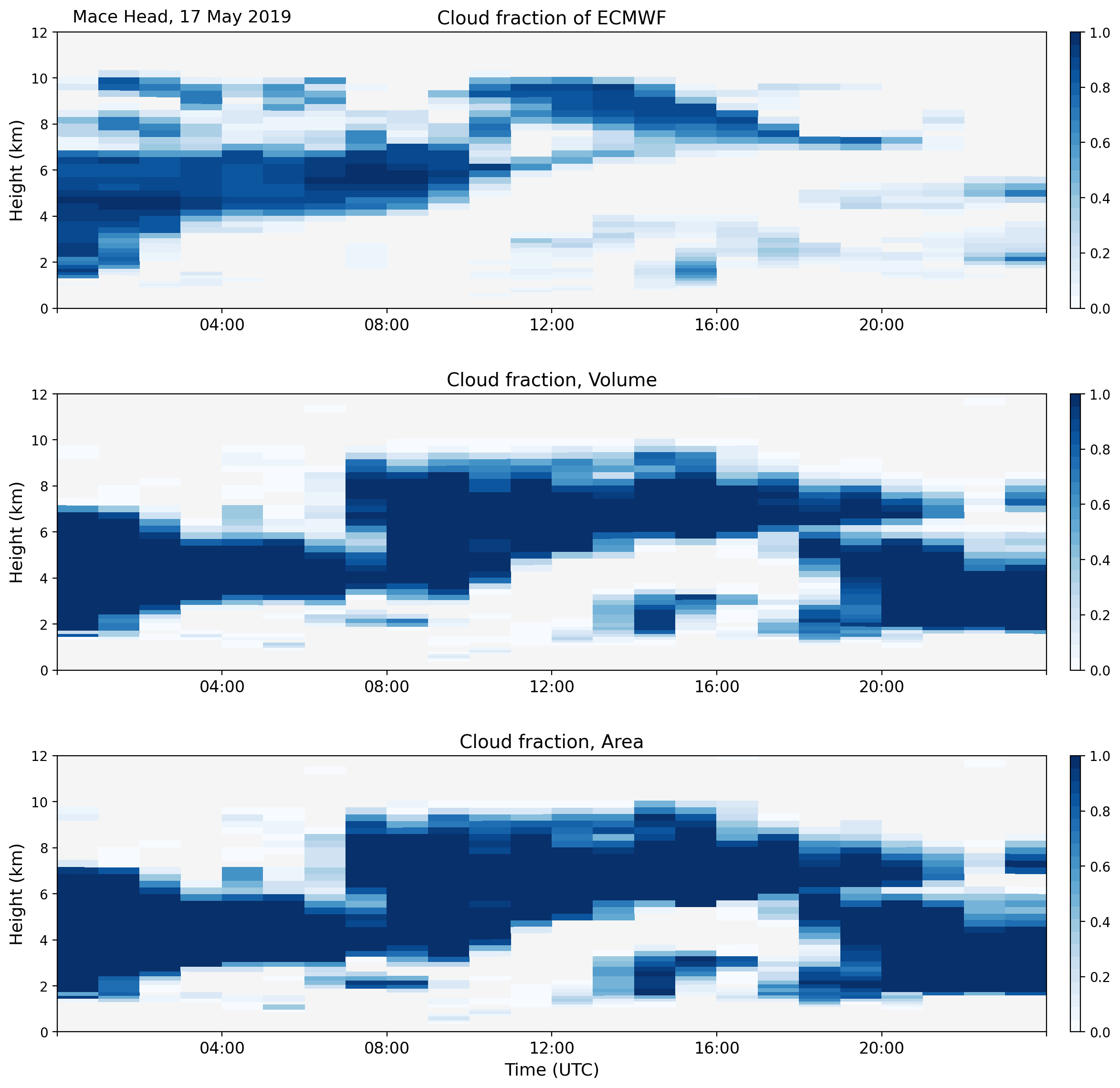
Observed and simulated cloud fraction. Model: ECMWF.

Observed and simulated IWC. Model: ECMWF.

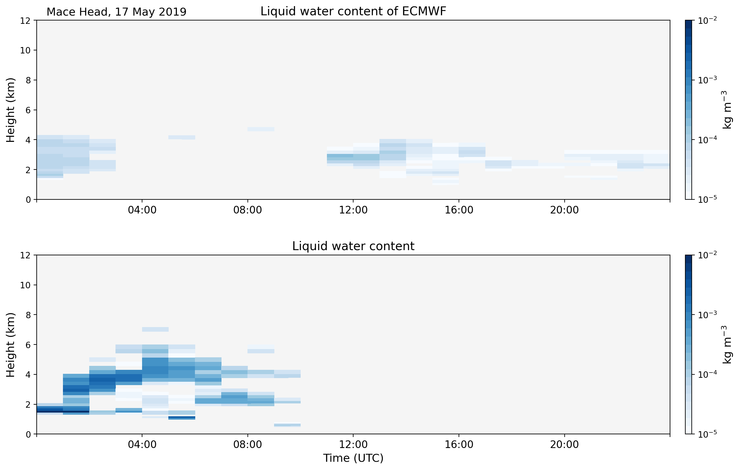
Observed and simulated LWC. Model: ECMWF.

Generating and plotting

Generate an L3 day product:

from cloudnetpy.model_evaluation import process_L3_day_product

process_L3_day_product(
    "ecmwf",          # model name
    "cf",             # product: "cf", "iwc" or "lwc"
    "ecmwf.nc",       # harmonized model file
    "categorize.nc",  # Cloudnet L2 observation product
    "l3-cf.nc",       # output file
)

Plot the result. The default group figure draws the model field and its downsampling methods as colormesh subplots, with the standard and advection time grids drawn into separate figures.

from cloudnetpy.model_evaluation import generate_L3_day_plots

# Colormesh group figure
generate_L3_day_plots("l3-cf.nc", "cf")

Supported models

The subpackage is model-agnostic: any model whose file has been harmonized to the common variable names and units can be evaluated. Models routinely used in Cloudnet processing include ECMWF, HARMONIE and ICON. The only model-specific handling is the optional summing of snow and graupel into the ice water content for models (such as HARMONIE) that do not keep all frozen mass in qi.