MWRpy processing

In this tutorial MWRpy products are generated from raw data, including quality control and visualization. This example utilizes files taken from the ACTRIS site Hyytiala equipped with a RPG-HATPRO instrument:

RPG microwave radiometer:
- Brightness temperatures: 230406.BRT
- Housekeeping data: 230406.HKD
- Elevation scans: 230406.BLB
- Weather station: 230406.MET
- Infrared radiometer: 230406.IRT

Note

.BRT and .HKD files are mandatory in MWRpy for processing

First step for the processing examples is to specify the site name and data path:

import os

site_name = "hyytiala"
package_dir = os.getcwd()
data_path = f"{package_dir}/tests/data/{site_name}"

E-PROFILE format

First E-Profile specific metadata can be configured in the instrument type configuration file (mwrpy/site_config/hatpro.yaml), which also includes instrument specific information. An optional site specific configuration file (e.g. mwrpy/site_config/{site_name}/config.yaml) can be configured, when dealing with multiple

instruments of the same type.

Level 1c

Now we convert RPG microwave radiometer (MWR) binary files, including brightness temperature (TB) and housekeeping data (*.BRT, *.HKD), into a Level 1c netCDF file (1C01, default). Data from optional elevation scans (* .BLB, *.BLS), weather station (*.MET) and infrared radiometer (*.IRT) are combined in this process and the following quality flags are derived:

Bit 1: missing_tb
Bit 2: tb_below_threshold
Bit 3: tb_above_threshold
Bit 4: spectral_consistency_above_threshold
Bit 5: receiver_sanity_failed
Bit 6: rain_detected
Bit 7: sun_moon_in_beam

Quality flags are stored as bits and Bit 1-3 include checks for missing brightness temperature values and their valid range (2.7 - 330 K). The spectral consistency flag (Bit 4) compares measured and retrieved TB. For this flag, it is expected to have the corresponding RPG retrieval coefficient file (SPC*.RET) in /mwrpy/site_config/{site_name}/coefficients/. Data from HKD files are used to determine the stability of the receiver components (Bit 5). The sensor from the attached weather station detects rain for quality Bit 6 and the sun and moon orbits are calculated and compared to the measurement geometry to detect potential interferences (Bit 7). A quality flag status variable contains information whether the flag is active.

from mwrpy.level1.write_lev1_nc import lev1_to_nc

mwr_raw = lev1_to_nc(
    data_type="1C01",
    path_to_files=data_path,
    data_format="e-profile",
    site=site_name,
    output_file=f"{data_path}/mwr_1c.nc",
)

The data format of the generated mwr_1c.nc file, including metadata information and variable names, is compliant with the data structure and naming convention developed in the EUMETNET Profiling Programme E-PROFILE.

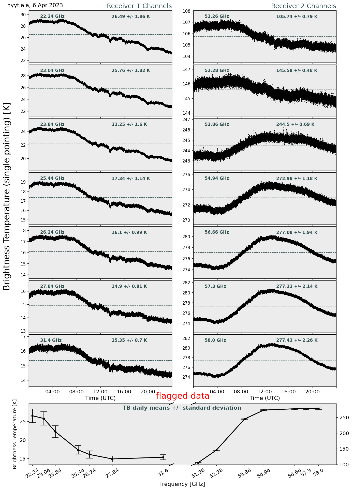
Variables such as brightness temperature can be plotted from the newly generated file.

from mwrpy.plots.generate_plots import generate_figure

generate_figure(f"{data_path}/mwr_1c.nc", ['tb'], save_path=f"{data_path}/")

Level 2 Single Pointing

Based on the Level 1c netCDF file mwr_1c.nc, MWR single pointing data are extracted and product specific retrieval coefficients (LWP*.RET, IWV*.RET, TPT*.RET, HPT*.RET, STA*.RET) are applied to generate the Level 2 single pointing product:

from mwrpy.level2.lev2_collocated import generate_lev2_single

mwr_prod = generate_lev2_single(
    mwr_l1c_file=f"{data_path}/mwr_1c.nc",
    output_file=f"{data_path}/mwr-single.nc",
    data_format="e-profile",
)

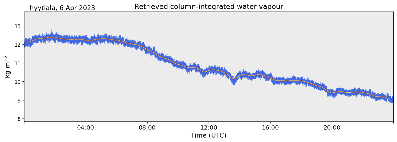
Variables such as integrated water vapor (IWV) can be plotted from the newly generated file.

from mwrpy.plots.generate_plots import generate_figure

generate_figure(f"{data_path}/mwr-single.nc", ['iwv'], save_path=f"{data_path}/")

Level 2 Multiple Pointing

Based on the Level 1c file, MWR multiple pointing data (elevation scans) are extracted and product specific retrieval coefficients (TPB*.RET) are applied to generate the Level 2 multiple pointing product:

from mwrpy.level2.lev2_collocated import generate_lev2_multi

mwr_prod = generate_lev2_multi(
    mwr_l1c_file=f"{data_path}/mwr_1c.nc",
    output_file=f"{data_path}/mwr-multi.nc",
    data_format="e-profile",
)

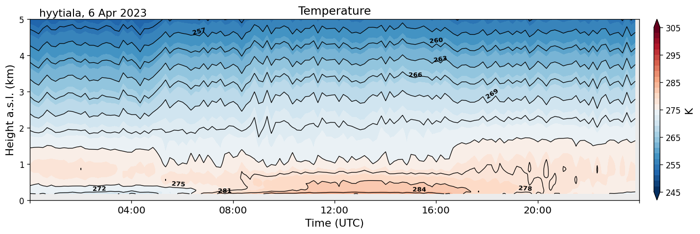
Variables such as temperature profiles can be plotted from the newly generated file.

from mwrpy.plots.generate_plots import generate_figure

generate_figure(f"{data_path}/mwr-multi.nc", ['temperature'], save_path=f"{data_path}/")

Cloudnet format

In this example the Cloudnet API client is used to fetch data and retrieval files and the Cloudnet data format is selected for processing (default).

Using Cloudnet API to fetch data and retrieval files

Download raw data (binary files):

from cloudnet_api_client import APIClient

date = "2023-04-06"
instrument_pid = "https://hdl.handle.net/21.12132/3.f360a2375f3e4e4f" # check https://cloudnet.fmi.fi/instruments to find the PID of your instrument
client = APIClient()
instruments = client.instruments()
i_type = [i.instrument_id for i in instruments if i.pid == instrument_pid][0]
files = client.raw_files(site_id=site_name, instrument_id=i_type, date=date)
binary_files = [f for f in files]

binary_filepaths = await client.adownload(binary_files, data_path)

Download retrieval files:

import requests

calibration = client.calibration(instrument_pid, date)
retrieval = calibration["data"]

retrieval_files = []
for file in retrieval["coefficientLinks"]:
    filename = f"{data_path}/{file.split('/')[-1]}"
    response = requests.get(file)
    with open(filename, "wb") as f:
        f.write(response.content)
        retrieval_files.append(str(filename))

Process and plot Level 1 data

In contrast to the E-PROFILE data format, no additional metadata needs to be defined in the configuration file. The fetched retrieval files are set as an argument together with site information (e.g. site name, altitude, etc.).

site_info = client.site(site_id=site_name)
site_meta = {
    "site": site_info.id,
    "altitude": site_info.altitude,
    "latitude": site_info.latitude,
    "longitude": site_info.longitude,
}

from mwrpy.level1.write_lev1_nc import lev1_to_nc
mwr_raw = lev1_to_nc(
    data_type="1C01",
    path_to_files=data_path,
    output_file=f"{data_path}/mwr_1c.nc",
    coeff_files=retrieval_files,
    instrument_config=site_meta,
)

In this example, the figure is only displayed and not saved.

from mwrpy.plots.generate_plots import generate_figure
fig_name = generate_figure(f"{data_path}/mwr_1c.nc", ['tb'], show=True)

Process and plot Level 2 data (single & multiple pointing)

Again, no plots are saved, only displayed.

from mwrpy.level2.lev2_collocated import generate_lev2_single
mwr_prod = generate_lev2_single(
    mwr_l1c_file=f"{data_path}/mwr_1c.nc",
    output_file=f"{data_path}/mwr-single.nc",
    coeff_files=retrieval_files,
)

from mwrpy.plots.generate_plots import generate_figure
fig_name = generate_figure(f"{data_path}/mwr-single.nc", ['iwv'], show=True)

from mwrpy.level2.lev2_collocated import generate_lev2_multi
mwr_prod = generate_lev2_multi(
    mwr_l1c_file=f"{data_path}/mwr_1c.nc",
    output_file=f"{data_path}/mwr-multi.nc",
    coeff_files=retrieval_files,
)

from mwrpy.plots.generate_plots import generate_figure
fig_name = generate_figure(f"{data_path}/mwr-multi.nc", ['temperature'], show=True)